***I provide ultrasonic transducer simulation services for product development. Please learn more about my consulting here: https://www.ultrasonicadvisors.com/***

In this article, we are going to demonstrate the electrical/impedance frequency response of a piezoelectric element using COMSOL. We will perform this using a 2D simulation. We will also be discussing phasor theory, how to use relevant expressions in COMSOL, apply boundary conditions, and how to determine and plot the impedance  and the phase .

SETTING UP THE SIMULATION

To start, go to COMSOL -> WIZARD -> STRUCTRURAL MECHANICS -> PIEZO. Next, Go to STUDY and select FREQUENCY RESPONSE.

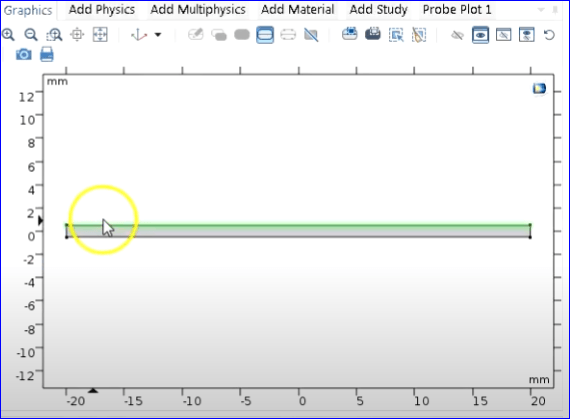
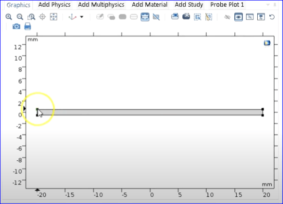
After setting this up, Select Rectangle as the Geometry.

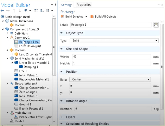
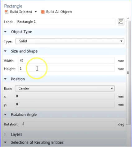
Change the unit to millimeters, and then create a rectangle with Width = 40mm and Height = 1 mm.

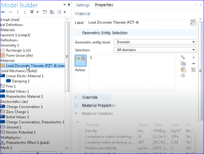
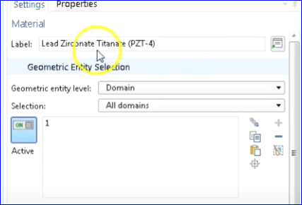
Select PZT-4 as the material.

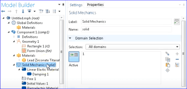
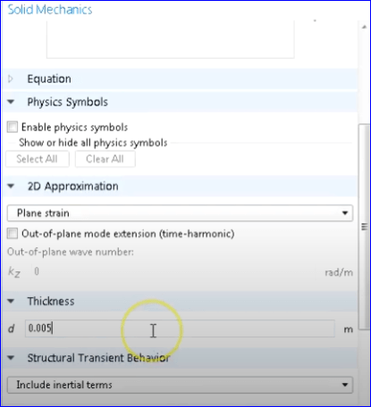
Under Solid Mechanics, set the thickness of the material to 0.005 m.

The thickness here is the out-of-plane thickness of the sample which is important for the mechanical response of the material. Although you won’t get stress distribution in that domain, it has effects on other parameters. 

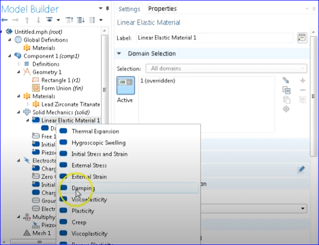
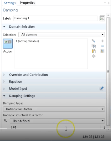
Under Linear Elastic Material, Select Damping. 

Select Isotropic as the Solid Model.

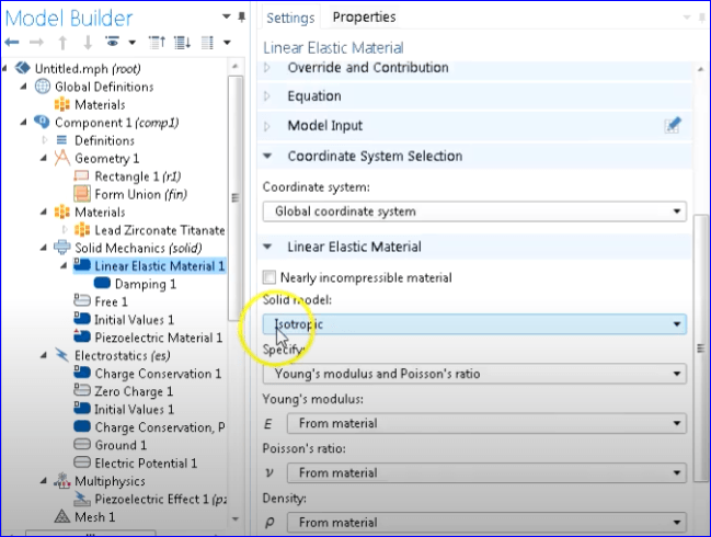
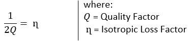
Set the Isotropic Loss Factor of the material which relates to the Quality Factor (Q) of the material.

Assuming a Quality Factor  Q = 500. Using this , we have the Equation:

Using the value  Q = 500, we have:

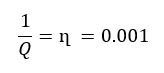
Ideally, we should set the Isotropic Loss Factor on COMSOL to the computed value 0.001, as that is close to the value for PZT-4. However, in this simulation, to be able to witness the effect of damping better, we will use a value of n = 0.01 instead. This translates to a Quality Factor Q = 50. A more typical representation of our software PZT such as PZT-5. 

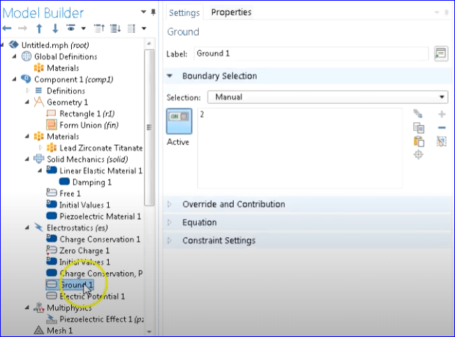
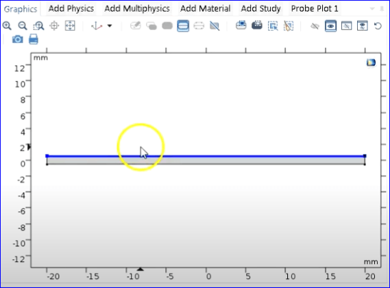
Specify the bottom of the plate as Ground.

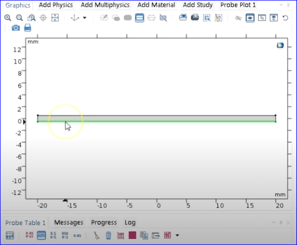
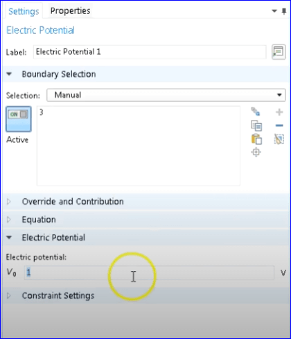
Specify the top of the plate as having Electric Potential.

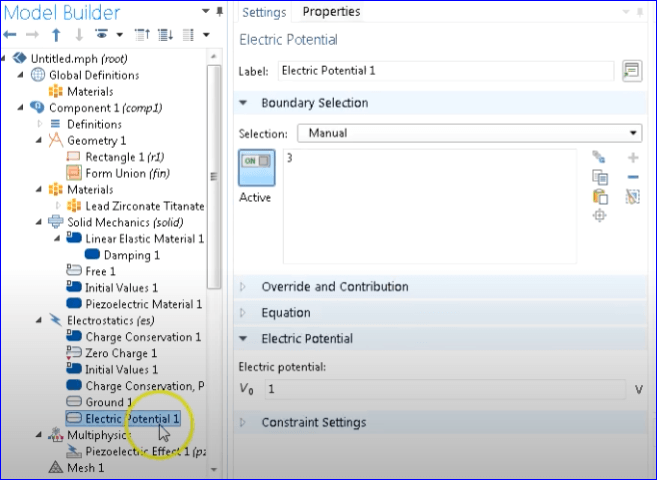
Set the Electric Potential to 1 Volt.

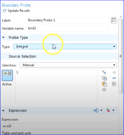
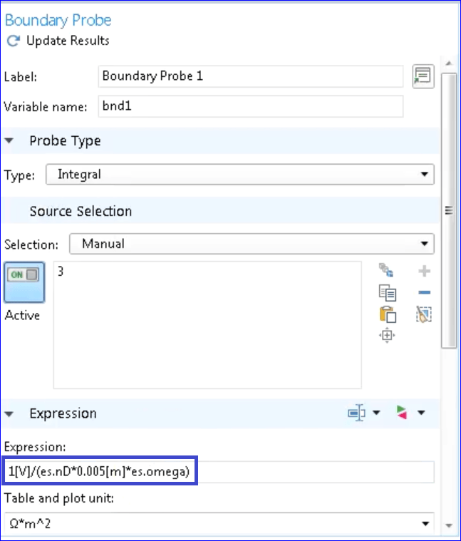
Apply Boundary Probe by going under Definition -> Probes -> Boundary Probe.

After creating Boundary Probe, select the top of the plate as the boundary.

Notice the unit of our expression, Charge per meter (C/m). 

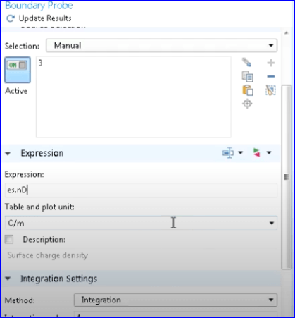
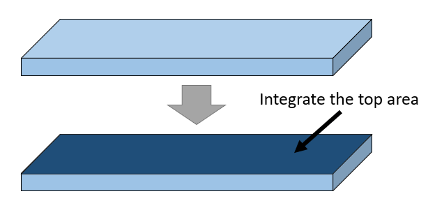
In case we have a 3D simulation, this unit will be Charge per square meter (C/m^2)  because that would be the electrode and the electrode is in 1D, therefore we have to integrate over that electrode. 

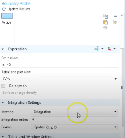
To be able to do this in COMSOL, select Integration as the Method and set the probe type as integral.

Normally, with a two dimensional electrode we use the formula :

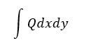
However, in our case, since the electrode is defined one dimension, we only have:

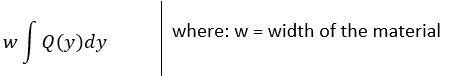
Based from our new equation, it means that we can already integrate the width by multiplying it.

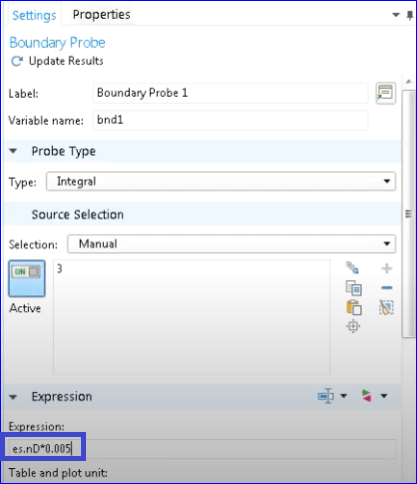
To reflect this on our COMSOL simulation, we multiply the expression with our set width which as defined earlier is 0.005 m.

At this point, we already know the total charge of the material. However, in most cases, we are more interested in the current.

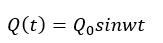
Using the equation of charge with respect to time, 

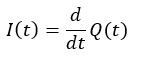
And since we know that the derivative of charge is equal to the current, we have the equation:

Simplifying the equation:

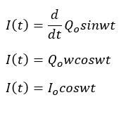
From the equation we can see that

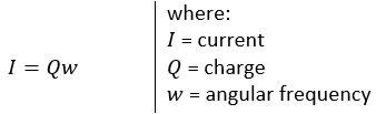
To reflect this to our COMSOL simulation, we should also multiply our expression by the angular frequency. Also to make sure that we get the units right, we will also specify the units in our expression.

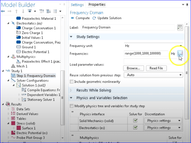
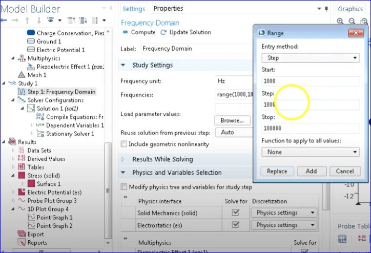
Under Frequency Domain, Set the Frequency Range Step to 1000.

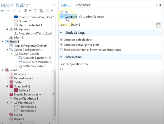
Now we have already finished setting up, we can now run the simulation by going to Study and press Compute.

ANALYZING SIMULATION RESULTS

In order to view the impedance and current response, select Probe Plot in the results.

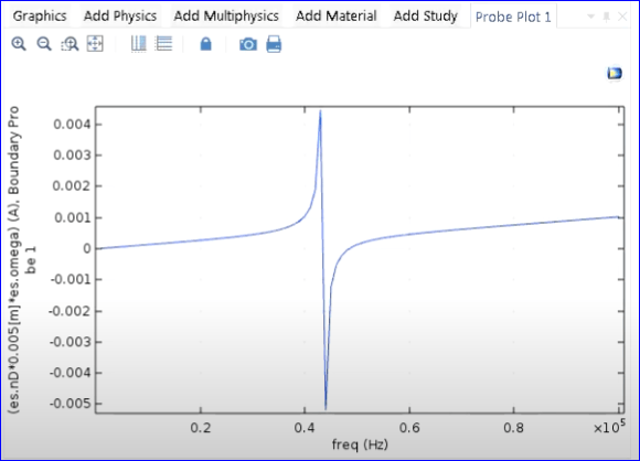
The figure shows the current response with respect to frequency.

We have both negative and positive current. We also have imaginary current which this is due to the fact that we have positive and negative phase. Only the real part of the current is being plotted here, however we need to plot amplitude and in order to plot amplitude we need to calculate the absolute value. 

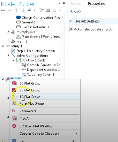
To do that in COMSOL, under Results create 1D Plot Group.

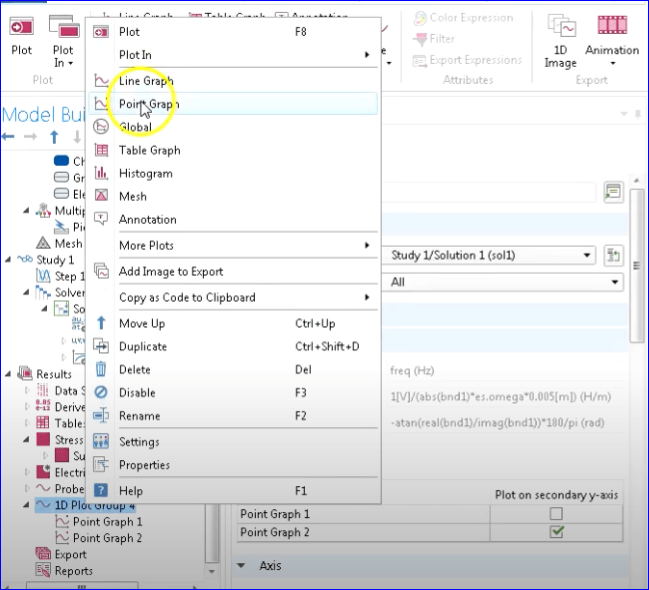
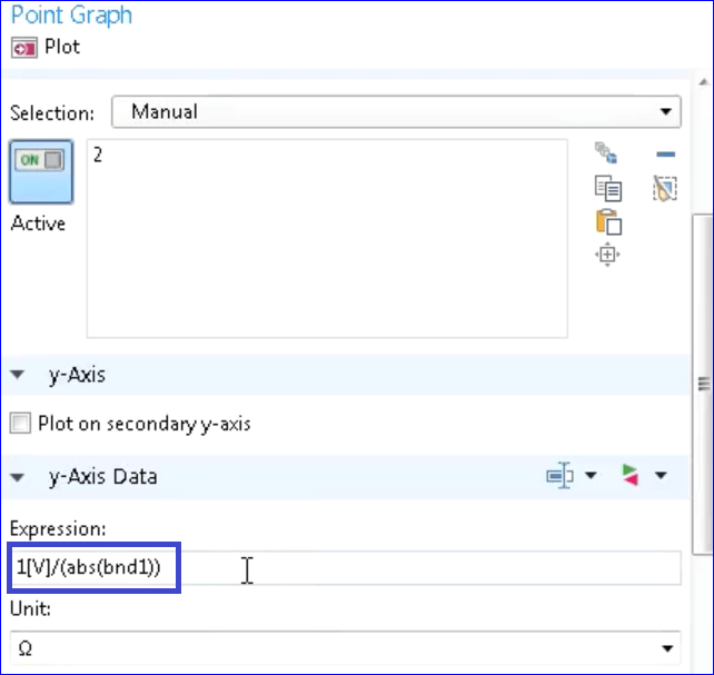
Under 1D Plot Group, create Point Graph.

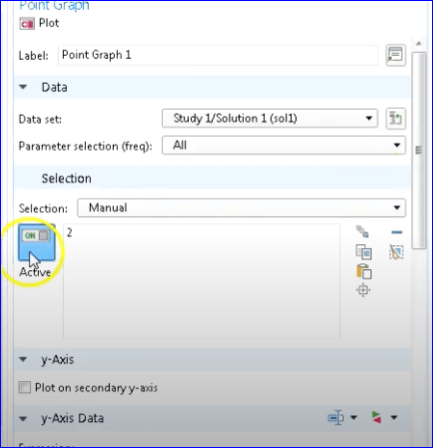
Set the Point Graph to Active and select a Point on the boundary we previously measured.

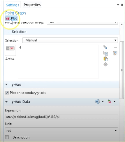
Type the corresponding expression for impedance.

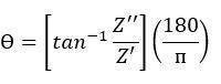
We also need an expression to calculate phase.

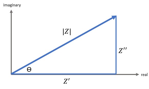
Using the diagram above, we have the Equation:

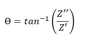
Converting the phase angle in degree we multiply the right side of the equation with the conversion factor:

It must also be noted that Impedance (Z) is inversely proportional to Current (I) .

And basically, bnd1 is proportional to the current.

That being said, we can also write the equation of phase in terms of current so we have:

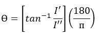
Reflect the corresponding equation in COMSOL expression.

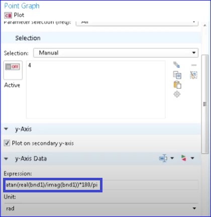
Plot the graph.

On the graph, we can see that the resonance and anti-resonance frequency is plotted on the negative side. 

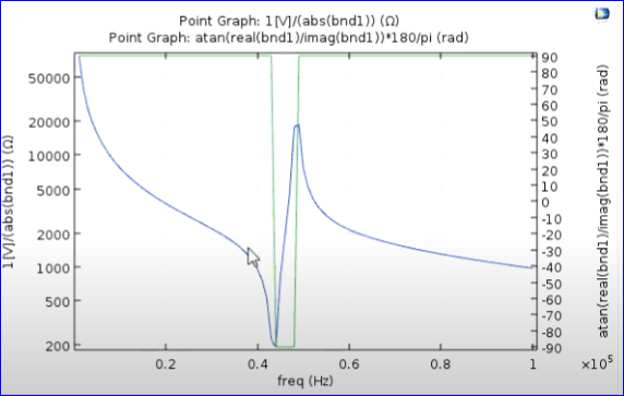
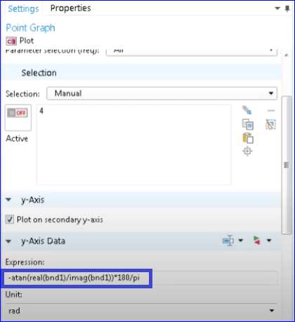
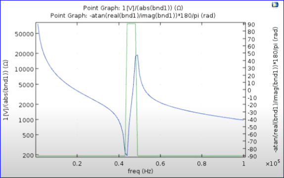
To compensate that, we simply negate our expression and plot again.

So basically that’s it, we are now able to show the electrical frequency response of a piezoelectric element using COMSOL. By including a finer frequency interval, we will be able to see the gradual change in phase and impedance around the resonance and antiresonance frequency. 

If you need help with simulation of your ultrasonic device in COMSOL or any other FEA package, please set up a free consultation with me at calendly.com/ultrasonicadvisors/30min or by emailing me at husain@ultrasonicadvisor.com

I advise to students and industry professional alike. Many of these discussions have resulted in full projects with Ultrasonic Advisors.